Trash segmentation with Yolo
Addressing the challenge of waste management is becoming increasingly important, and technology is playing a key role in making this process more efficient. In this article, we’ll explore how to build a trash segmentation algorithm using YOLO (“You Only Look Once”), a fast and accurate object detection model, alongside TACO (Trash Annotations in Context), a dataset designed specifically for trash detection.
We’ll discuss how the TACO dataset aligns with the widely-used COCO dataset format and guide you through the necessary steps to convert the data for compatibility with YOLO’s segmentation training. After that, we’ll demonstrate how to train the YOLO-seg model on Google Colab, a cloud platform that provides powerful GPUs without requiring local hardware. Finally, we’ll analyze the results to evaluate the performance and practical insights from the model.
If you’re interested in applying AI techniques to environmental challenges, this article offers a clear and practical walkthrough of creating an effective trash segmentation system.
Yolo
YOLO (You Only Look Once) is a family of real-time object detection models that frame detection as a single regression problem, predicting bounding boxes and class probabilities directly from the input image in one pass. This approach makes YOLO extremely fast and efficient compared to two-stage detectors, while still maintaining good accuracy.
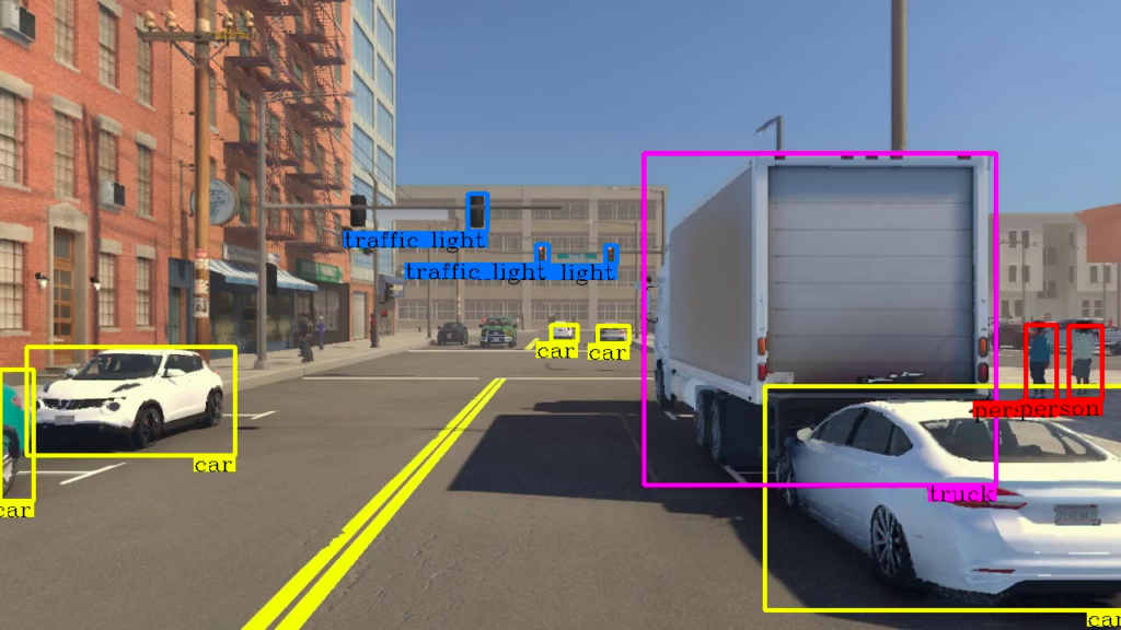
Recent versions of YOLO extend beyond bounding box detection to support instance segmentation, where the model not only identifies the location and class of an object but also generates a precise pixel-level mask. This capability is particularly useful in scenarios that require detailed shape information, such as medical imaging, robotics, and industrial quality inspection. YOLO segmentation combines the speed of the original architecture with the fine-grained output of segmentation models, making it a practical choice when both accuracy and efficiency are critical.
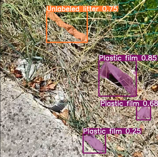
Yolo dataset format
Ultralytics expects a very simple layout: images and labels live in parallel folders, and every image has a text file with the same name containing one line per object.
datasets/taco-yolo/
├── data.yaml
├── images/
│   ├── train/   0001.jpg, 0002.jpg, ...
│   └── val/     0101.jpg, ...
└── labels/
    ├── train/   0001.txt, 0002.txt, ...
    └── val/     0101.txt, ...
For segmentation, each line of a label file describes one instance as a class index followed by the vertices of its polygon:
<class> <x1> <y1> <x2> <y2> ... <xn> <yn>
All coordinates are normalized between 0 and 1 (divided by the image width and height), and the class index starts at 0. An image with no objects simply gets an empty file, or no file at all. A bounding-box label, in contrast, has only four numbers: <class> <x_center> <y_center> <width> <height>. That is why a segmentation dataset can always be turned into a detection one, but not the other way round.
The data.yaml file tells the trainer where everything is and how the classes are named:
path: datasets/taco-yolo
train: images/train
val: images/val
names:
  0: bottle
  1: can
  2: cigarette
  # ...
TACO
TACO (Trash Annotations in Context) is an open image dataset of litter in the wild, built by Pedro Proença and Pedro Simões. Its photos were taken in very different places: streets, parks, woods and beaches. They show trash lying on grass, sand, asphalt or in water, which makes the problem hard and the data realistic. That’s the main difference from many waste datasets, where a single clean object sits on a plain background.
Some numbers about the official release:
- about 1,500 images and 4,800 annotated objects;
- 60 categories (bottle, can, cigarette, plastic bag, bottle cap, straw…) grouped into 28 super-categories;
- every object has a pixel-level polygon mask drawn by hand, not just a box;
- an open project: anyone can contribute new photos and annotations through the website.
The dataset is small compared with COCO, and very unbalanced: a few classes such as cigarettes, plastic film and bottle caps account for most of the instances, while many others have only a handful of examples. Keep this in mind, because it shapes the whole training stage.
TACO dataset format
TACO ships in COCO format: a single annotations.json file describes every image and every object, while the pictures are downloaded separately by a script, since they come from Flickr and other sources. The JSON has three main lists:
{
  "images": [
    {"id": 0, "file_name": "batch_1/000006.jpg", "width": 1537, "height": 2049}
  ],
  "annotations": [
    {
      "id": 0, "image_id": 0, "category_id": 6,
      "segmentation": [[561.0, 1238.0, 590.5, 1190.0, 640.0, 1203.0, ...]],
      "bbox": [561.0, 1190.0, 183.0, 214.0],
      "area": 21090.0, "iscrowd": 0
    }
  ],
  "categories": [
    {"id": 0, "name": "Aluminium foil", "supercategory": "Aluminium foil"}
  ]
}
COCO and YOLO describe the same ground truth with different conventions:
| COCO (TACO) | YOLO | |
|---|---|---|
| Files | one JSON for the whole dataset | one .txt per image |
| Coordinates | absolute pixels | normalized 0–1 |
| Box | [x_min, y_min, width, height] |
[x_center, y_center, width, height] |
| Polygon | [[x1, y1, x2, y2, ...], ...], possibly several rings |
one flat list on a single line |
| Class ids | arbitrary integers (id) |
contiguous indices from 0 |
TACO dataset convertion
Converting means reading the JSON once, grouping the annotations by image, normalizing each polygon and writing one text file per image. A few details are easy to get wrong:
- Class ids must be contiguous. TACO category ids can have gaps, so we build an explicit mapping to indices
0..N-1. - One annotation can contain several polygons (an object partially hidden by something else). Each ring becomes its own line.
- Degenerate polygons must be dropped. A polygon needs at least three points, and a few TACO masks are too small to be useful.
- Split by image, never by object, otherwise the same photo ends up in both training and validation, and the validation score becomes meaningless.
- Phone photos carry EXIF rotation. If a viewer applies it and the annotation tool did not (or vice versa), masks end up rotated. Check a few labelled images by eye before training.
import json
import random
import shutil
from collections import defaultdict
from pathlib import Path

SRC = Path("TACO/data")                 # images + annotations.json
DST = Path("datasets/taco-yolo")
VAL_FRACTION = 0.15

coco = json.loads((SRC / "annotations.json").read_text())

# TACO category ids -> contiguous YOLO class indices
categories = sorted(coco["categories"], key=lambda c: c["id"])
class_index = {c["id"]: i for i, c in enumerate(categories)}

images = {im["id"]: im for im in coco["images"]}
polygons = defaultdict(list)             # image_id -> list of label lines

for ann in coco["annotations"]:
    im = images[ann["image_id"]]
    w, h = im["width"], im["height"]
    for ring in ann["segmentation"]:
        if len(ring) < 6:                # fewer than 3 points
            continue
        coords = []
        for x, y in zip(ring[0::2], ring[1::2]):
            coords += [min(max(x / w, 0), 1), min(max(y / h, 0), 1)]
        line = " ".join(f"{v:.6f}" for v in coords)
        polygons[im["id"]].append(f"{class_index[ann['category_id']]} {line}")

# Split by image
ids = sorted(images)
random.Random(42).shuffle(ids)
n_val = int(len(ids) * VAL_FRACTION)
split = {i: ("val" if k < n_val else "train") for k, i in enumerate(ids)}

for image_id, im in images.items():
    part = split[image_id]
    name = Path(im["file_name"]).with_suffix("").as_posix().replace("/", "_")
    (DST / "images" / part).mkdir(parents=True, exist_ok=True)
    (DST / "labels" / part).mkdir(parents=True, exist_ok=True)
    shutil.copy(SRC / im["file_name"], DST / "images" / part / f"{name}.jpg")
    (DST / "labels" / part / f"{name}.txt").write_text("\n".join(polygons[image_id]))

names = "\n".join(f"  {i}: {c['name']}" for i, c in enumerate(categories))
(DST / "data.yaml").write_text(
    f"path: {DST.resolve()}\ntrain: images/train\nval: images/val\nnames:\n{names}\n"
)
A last sanity check is worth five minutes: load a handful of converted images, draw their polygons on top, and make sure the masks sit on the objects. Most training problems that look like “the model doesn’t learn” turn out to be label problems.
Yolo-seg training
Training runs on Google Colab with a free GPU (a T4 is enough for the small models). After mounting Drive, so the checkpoints survive a disconnection, the whole training fits in a few lines thanks to the Ultralytics API:
from ultralytics import YOLO

model = YOLO("yolo11n-seg.pt")           # pretrained on COCO, segmentation head

model.train(
    data="/content/datasets/taco-yolo/data.yaml",
    epochs=100,
    imgsz=640,
    batch=16,
    patience=20,                          # stop early if validation stops improving
    project="/content/drive/MyDrive/taco",
    name="yolo11n-seg",
)
Some choices worth explaining:
- Start from pretrained weights.
yolo11n-seg.pthas already learned edges, textures and shapes on COCO, so TACO’s 1,500 images are used to specialise it rather than to teach it vision from scratch. Training from scratch on such a small dataset would overfit almost immediately. - Pick the model size by budget. The nano model trains in minutes and is small enough to run in real time even on embedded boards. Larger variants (
s,m,l) are more accurate on small objects such as cigarette butts, at the cost of memory and speed. - Image size matters for litter. Many objects are tiny in the frame. Increasing
imgszhelps, but quadruples the compute every time you double it. - Data augmentation is built in. Ultralytics applies mosaic, flips, scaling and colour jitter by default, which is very useful with so few images.
- Watch the validation curves.
patienceends the run when the validation metrics stop improving, and the best checkpoint is saved asbest.pt.
Results
I have to be honest: this experiment is unfinished. I didn’t get to a full training of the model on all 60 TACO categories with a proper evaluation, so I can’t give you reliable benchmark numbers, and I prefer not to publish any I can’t stand behind.
What I did manage is to train the model on the specific case I was interested in and verify that it works. The model learned to find and outline the target objects in that scenario. I haven’t measured how well it generalizes, so take this as a proof of concept rather than a performance claim. For a prototype this is the main result: the pipeline described above (COCO annotations, conversion to YOLO format, fine-tuning of a pretrained yolo11-seg model on Colab) works from end to end.
What is still missing to call it complete:
- A proper evaluation on a held-out set, with box and mask mAP50 and mAP50-95 for every class, not only on the case I trained for.
- Handling class imbalance. Rare categories need either more data, merging into the 28 super-categories, or class weighting, otherwise the model mostly learns the frequent ones.
- More data from the target environment. TACO is a great starting point, but a model deployed in a specific setting benefits enormously from a few hundred photos taken there.
- Export and deployment. Converting the best checkpoint to ONNX or TensorRT and measuring latency on the hardware where it will actually run.
If you try the pipeline yourself, I’d love to hear how it goes. Everything here is meant to be a starting point, and the missing steps are the natural next articles.